Gene-environment interaction analysis of school quality and educational inequality

Data

We use linked microdata from Statistics Netherlands (CBS) covering the whole population. We construct a dataset including twin families with information on children’s educational performance, school environment, and family SES. To construct twin families, we rely on basic demographic information on children and their legal parents, using linked parent-child data (KINDOUDERTAB, see ref. 68) combined with the municipal personal records database (GBAPERSOONTAB, see ref. 69). We identify families based on children who share the same legal parents. After constructing families, we identify twin pairs. Since the birth day is not available because of privacy reasons, we base this on children who have the same birth month and year. Based on the sex composition, we identify same-sex (SS) and opposite-sex (OS) twin pairs. Multiple twin pairs in one family are analytically complex. Therefore, we select one random twin pair in these cases.

We use the Cito database (CITOTAB, see ref. 70) to obtain information on educational performance. These data are available for 2006–2019 (birth cohorts 1994–2007) at the time of this study. Primary schools can permit Cito to share the data with the CBS, who anonymized the data and assigned identification numbers to link the data at the individual and school level. Data sources on parental SES that we use to construct school SES are the highest education database (Hoogsteopltab, see ref. 71) for the year 2018 and personal income for the period 2003–2018 (IPI for 2003–2015 and INPATAB for 2011–2018, see ref. 72). Data on educational attainment are largely based on diverse registrations of individuals who completed their education at an educational institution funded by the government. There is no (reliable) register data available for privately funded education (which is relatively rare in the Netherlands), education abroad, and long-term corporate training. To add information on this, the CBS used data from the Labor Force Survey which is collected on a sampling basis. Income data is based on administrative information, mostly provided by the tax authorities.

We supplement children and parent data from CBS with official information on the school environment obtained from the Dutch Inspectorate of Education and the Dutch Education Executive Agency. Inspectorate of Education data include many indicators that are used to assess the quality of schools by the inspectorate and are generally available from 1999 onward. Education Executive Agency data include information on general school characteristics such as the number of students and teachers. These data are (mostly) available from 2011 onward. School data can be linked to the CBS data via a school identifier (BRIN). This research was approved by the Ethics Committee of the Faculty of Social and Behavioral Sciences, Utrecht University (FETC20-216). Given the usage of administrative data, informed consent is not applicable.

Selections and selectivity

Figure 3 shows the sample selection. We only study twins from birth cohorts 1994–2007, due to data availability of our dependent variable. Only twin pairs for whom at least one twin has information on educational performance are included. One reason for the missingness is that some schools did not permit to share the results with CBS. Another reason is that schools can choose to administer another test. Most schools use the Cito test. Until recently, around 80% of the schools administered this test and these schools did not differ from the total school population regarding region, school size, urbanization, and percentage of students from low-educated families⁷³. For the most recent years, the percentage of schools administering the Cito test decreased (63.8% in 2017/2018, 55.9% in 2018/2019) and became a bit more selective. Schools in more urbanized areas and larger schools more often administered the Cito test^73,74. Excluding these years did not substantially change our results.

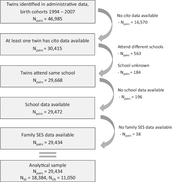
SS same-sex twin pairs, OS opposite-sex twin pairs.

We only include twins who went to the same primary schools. Most twins (in our data 98%) go to the same school. Those who attend different schools form a selective group (e.g., one twin attends a school for special needs). For 6415 twin pairs, at least one of the twins had missing information on the school identifier. In most of these pairs (6234 pairs), there was a co-twin with non-missing information. In these cases, we assume that both twins attended the same school. We exclude the twin pairs where both twins had missing information on school data. We also exclude twin pairs with missing information on parental SES. This leads to our analytical sample of N_pairs = 29,434.

Measurements

We measure our dependent variable, educational performance, by students’ scores on the Cito test. We use the most recent score in case of multiple observations, which may occur if children repeat the grade when the test is taken. The Cito test is a nationwide standardized educational achievement test taken at the end of primary education around age 12. It consists of multiple-choice items on Dutch language, mathematics, study skills, and world orientation (e.g., geography, biology, and history). The domains are combined into a standard score. Because the subdomain world orientation is not mandatory, this is not included in the standard score. The standard score is calculated based on the correctly answered questions with a formula taking into account the difficulty of the test for that year, to make the scores comparable over the years. It is aimed to have questions of a difficulty level between 0.40 and 0.90 with an average of around 0.70, where the difficulty level refers to the proportion of pupils who answered the item correctly⁷³. Another property of the Cito score is that the number of correct answers is transformed into a scale from 501–550, with a national average of 535 and a standard deviation of 10. If the scores are below 501 or above 550, they are rounded to the minimum or maximum⁷³. There is more censoring at the upper end than at the lower end of the scale. These properties of the scaling result in a somewhat negatively skewed distribution, although the skewness value of −0.6 does not suggest severe skewness. Also, the level of censoring is relatively low, with around 4% of twins obtaining the maximum score of 550. However, censoring occurs more among high-SES children (and thereby also more frequently in high-SES and high-quality schools). High-SES children more often obtain the maximum score, while obtaining the lowest score is uncommon. This pattern is also found in similar studies (see, e.g., refs. ^44,75) and has the consequence that gene-environment interactions may be (partly) due to a ceiling effect. We expect this to be a limited problem in our study. Both the Cito score and the (uncensored) raw test score show decreasing variance with increasing parental SES (see Supplementary Fig. 7). Also, a prior study investigating gene-family SES interactions in Cito scores shows that correcting for censoring did not change the results⁴⁴. Hence, it is unlikely that the decreasing variance with increasing parental SES (and the associated measures school SES and school quality) is solely driven by the censoring of the Cito scale.

For our moderator school quality, we construct a factor score based on data from the Inspectorate of Education. The Inspectorate data consist of many official indicators that are used to assess the quality of schools. These are generally available for the period 2000–2011, and sometimes up to 2019. Initially, we also included data from a second data source, namely, data from the Education Executive Agency. However, in the end, the indicators derived from these data (e.g., financing, number of pupils and staff) were not included in our measurement model due to low correlations with the other indicators or low factor scores (see Supplementary information Appendix E). The inspectorate data are not collected for scientific research purposes, but to assess whether schools meet a certain quality standard. The inspectorate usually visited schools once every four years, and the set of indicators that were used differed over the years. Although this provides a rich source of information, these data are not directly suited for research and require extensive data handling. The structure of the Inspectorate data with the resulting missing data makes it impossible to measure school quality per year or even a couple of years. Therefore, for each indicator, we take the average of all available years. Items are mostly measured on a three-point scale (insufficient, sufficient, good) or a four-point scale (bad, insufficient, sufficient, good). Sometimes, also a two-point scale is used (insufficient, sufficient; no, yes).

We construct factor scores based on the standardized items using factor analyses with Full Information Maximum Likelihood (FIML) estimation in Mplus. We conduct two Exploratory Factor Analyses (EFA): one for all the items related to school resources leading to two dimensions, and one for school climate leading to seven dimensions. Altogether, this leads to nine dimensions of school quality: (1) range of educational activities, (2) (implementation of) school curriculum, (3) guidance of educational needs, (4) parental involvement, (5) monitoring and evaluating (special needs) students, (6) learning climate, (7) social climate, (8) safety, (9) quality assurance (see Supplementary Tables 6, 7). Based on these dimensions, we construct one overall school quality factor in a third (confirmatory) factor analysis. The dimensions of social climate, parental involvement, and safety have a low loading on this overall factor (Supplementary Table 8) and/or a low correlation with schools’ average Cito score (Supplementary Table 9). As an alternative operationalization, we exclude these dimensions and construct a factor score based on the remaining six dimensions. This does not lead to substantially different results and therefore we keep all the dimensions in. Given the numerous latent variables and items, it is not possible to integrate the full measurement model with our analytical model. Therefore, we save the factor scores and include these in our analytical model as a single variable while imposing a measurement error correction. More information on this correction – as well as further details on the procedure, items, and factor analyses – are provided in the Supplementary information (Appendix E).

Parental SES is measured by a factor score based on parental education and income. For parental education, we use the father’s and mother’s highest attained level of education, which is coded according to the International Standard Classification of Education (ISCED) 2011. We rely on the most recent data file from 2018. For income, we use the father’s and mother’s percentile scores of personal yearly income for the year before the Cito test. Personal income includes the gross income from labor, own company, income insurance benefits, and social security benefits (excluding child benefits and child-related budget). Premiums for income insurance have been deducted. For the percentile score, personal income is divided into 100 equal groups of people with income in private households. We construct a factor score for SES based on standardized items using CFA in Mplus (see Supplementary information Appendix F). FIML is used to handle missing data, which is especially present for parental education (Supplementary Table 11). Data on parental income is also sometimes missing (for the father’s and mother’s income in 5% and 12% of the cases, respectively). We have income data on fathers and mothers who no longer form a household. Hence, missing values are not caused by a divorce or separation but the result of a combination of unknown causes. These potentially include a deceased parent, a migrated parent, a parent without income, or a data registration problem. Given the unknown causes and relatively small amount of missing, using FIML estimation in the parental SES measurement model is a suitable solution.

School SES is an aggregate of parental SES. We use the average parental SES of all children in the school who took the Cito test in the year that the twins took this test.

We control for year of birth and sex (0 = female, 1 = male) in all models. Descriptive statistics of all variables are presented in Table 3.

Twin method

In the classical twin design, structural equation modeling (SEM) is used to decompose the variance in a characteristic into three latent components. First, there is a component capturing additive genetic variance (A). This component partly reflects genetically influenced traits that positively influence educational performance, including cognitive ability but also non-cognitive traits such as self-efficacy and grit⁷⁶. It also captures genetic variance related to traits that negatively influence performance, for example, ADHD, depression, and antisocial behavior^20,77. Second, there is a common or shared environmental variance (C) component, which includes all environmental aspects making twins more alike such as influences of family resources, parenting practices, educational expectations, and the broader environmental context that differs between families⁴⁰. We use the C-component as a comprehensive measure of family background influences, reflecting social inequality in educational performance. Last, there is unique, non-shared, environmental variance (E), capturing aspects that make twins dissimilar. These include, for example, subjective experiences, differential treatments, luck, and measurement error²¹. Latent components A, C, and E are set to a variance of 1. Path coefficients a, c, and e represent the effects of the latent factors on educational performance. The variance is equal to the square of the path coefficient; hence the ACE model can be written mathematically as

where \({V}_{{educ}}\) is the total variance of our phenotype educational performance. We extend this model by including a continuous moderator (M)⁷⁸. In our case, our moderator school quality affects the average educational performance as shown by \(\mu +{b}_{m}M\). It could also moderate, for example, a to become \(a+{b}_{a}M\) (see Fig. 4). The total variance in this moderation model changes to

Latent variables represent genetic (A), shared-environmental (C), and non-shared environmental (E) components of educational achievement, with corresponding path coefficients (a, c, e). Measured variable M refers to the moderator. Genetic covariance for same-sex (SS) twin pairs is estimated by \({{rSS}}_{G}=1\frac{{N}_{{SS}}-{N}_{{OS}}}{{N}_{{SS}}}+0.5\frac{{N}_{{OS}}}{{N}_{{SS}}}\) = 0.70 and is 0.50 for opposite-sex (OS) twin pairs. We also use 0.75 and 0.80 as alternative values for rSS_G.

Parameters in this model are usually identified because zygosity is available. Identical (i.e., monozygotic; MZ) and fraternal (i.e., dizygotic; DZ) twins differ in genetic resemblance: where MZ twins are genetically identical at conception, DZ twins share on average half of their segregating genes. Hence, the genetic correlation (A1–A2) can be constrained to 1 for MZ twins and 0.5 for DZ twins. It is assumed that MZ and DZ twins share their environment to the same extent, meaning that shared environmental correlation (C1–C2) can be constrained to 1 for both MZ and DZ twins. Accordingly, the MZ covariance is \({{Cov}}_{{mz}}={V}_{A}+{V}_{C}\) and for DZ twins this is \({{Cov}}_{{Dz}}={0.5V}_{A}+{V}_{C}.\)

Constraining the shared environmental variance to be equal reflects the Equal Environment Assumption (EEA). Violation of the EEA could overestimate A and underestimate C, but only if differential treatment is related to the outcome under study. Several studies showed that the EEA is unproblematic for a wide range of outcomes⁷⁹, including school performance specifically^80,81. Additional assumptions are no assortative mating, generalizability of twins to the general population, minimal gene-environment correlation, and absence of non-additive genetic effects. Violations of these assumptions could bias A and C but do so in different directions⁸². These consequences of violations (upward or downward bias of A and C) are reflected in the difference in genetic relatedness between twin types. We perform the analyses with different genetic correlations to test to what extent our results are sensitive to the assumptions.

Twin model with unknown zygosity

We do not have information on zygosity but instead rely on data from 18,384 same-sex (SS) and 11,050 opposite-sex (OS) twin pairs. OS twins are always DZ, hence their genetic correlation (A1–A2) is equal to 0.5. SS twins are a mixture of MZ and DZ twins. The true value for the average genetic correlation of SS twins (i.e., rSS_G) is unknown, and there are different ways in the literature to deal with this^32,83,84. A common way is using Weinberg’s differential rule to estimate the proportion of MZ and DZ twins within SS twin pairs⁸⁵. According to this rule, the probability of male births equals the probability of female births, and therefore among DZ twins the number of SS twins equals the number of OS twins. The total number of DZ twins is thus twice the number of OS twins. The proportion of MZ twins within SS pairs in our data can be estimated by \({p}_{{MZSS}}\) = (N_SS – N_OS) / N_SS = (18,384–11,050) / 18,384 = 0.40. For DZ twins within SS pairs this is \({p}_{{DZSS}}\) = 1 – 0.40 = 0.60. This leads to an average genetic relatedness among SS twins of rSS_G = (1*0.40) + (0.5*0.60) = 0.70. Another common approach, which is based on the assumption that among SS twins half will be MZ and half will be DZ, is to use \({{rSS}}_{G}\) = 0.75 (i.e., the average genetic relatedness of MZ and DZ twins)⁸⁴.

While the MZ twin rate is relatively stable over time and MZ twinning is thought to be the result of a random event, this is not the case for DZ twins. DZ twin births are related to individual characteristics (DZ twin pregnancies are more common when the mother is older, taller, has a higher BMI, and smokes, among others) and the usage of assisted reproductive technology (ART) such as in vitro fertilization (IVF)⁸⁶. There are also indications that the usage of ART is related to MZ twin pregnancies, but the underlying causes are unknown^86,87. In the Netherlands, the average maternal age and use of ART increased over the past decades, although the IVF policy has become more conservative (increasingly only one embryo is being transferred)⁸⁶. Assuming a fifty-fifty mixture of MZ and DZ twins among the SS pairs is likely not realistic for the population that we study. Relying on the estimated genetic relatedness using Weinberg’s differential rule overcomes this problem. Indeed, when we calculate the MZ/DZ ratio among SS twins we find a larger share of DZ twins among SS twins (i.e., a ratio of 40/60, leading to the estimated genetic relatedness of rSS_G = 0.70).

Relying on a twin model with unknown zygosity has been criticized⁸⁸. One concern is that the design is less powerful than using information on zygosity. This is less applicable to our study given the use of population data. Another concern is that the method relies on the assumption that the correlation of SS twin pairs only differs from that of OS twin pairs because SS twins are on average genetically more similar, not for other non-genetic reasons³². This assumption is violated if SS DZ twins are more similar to one another than OS DZ twins because the first are from the same sex and the latter are not. One could test this by comparing intraclass correlation coefficients (ICCs) of SS and OS pairs with known zygosity. This has been done for reading and mathematics achievement using data from the Netherlands Twin Register⁴⁵. Comparing the similarity in educational achievement for SS and OS pairs and MZ and DZ pairs with different sex compositions demonstrated that the assumption holds⁴⁵. Another way to test this is by comparing the ICCs of SS and OS non-twin sibling pairs. This shows that SS siblings are slightly more similar (average ICC for males and females = 0.44) than OS siblings (ICC = 0.42), suggesting small sex influences (Supplementary Fig. 8).

Although the difference is only 0.02, it could still lead to a non-negligible upward bias in estimates of genetic variance and a downward bias in shared environmental variance. To give an intuition for the possible size of the bias, if one uses the ICC of OS DZ twins (0.45), the descriptive estimate of heritability would be 0.80, which can be calculated with the formula (ICC_SS –ICC_OS) / (rSS_G – rOS_G) = (0.61–0.45) / (0.70–0.50). If we assume that the sex-effect for twins is the same as for non-twin siblings, the ICC for SS DZ twins would be 0.45 + 0.02 = 0.47. Based on this ICC, heritability would be 0.70. One can correct this bias by using a larger value for rSS_G. Note that theoretically, one would adjust the shared environmental correlation of OS twins downwards to consider that their environments are less similar because they are of different sexes. However, genetic and shared environmental relatedness account for the same pattern in the data (cf. Spinath et al. 2004), so it makes sense to only adjust one at a time. Practically, increasing rSS_G is similar to decreasing the shared environmental correlation of OS twins. We, therefore, perform our analyses using three values of rSS_G (0.70, 0.75, 0.80). As we will show, our conclusions are robust to the different values.

Analytical strategy

We fit a series of ACE models in Mplus. We have data on 29,434 twin pairs nested in 5843 schools. To account for this nested structure, we adjust the standard errors for clustering at the school level. In all models, the influences of sex and birth year are controlled for by including them as covariates. We z-standardize all continuous independent variables prior to the analyses. Before fitting the twin models, we test for equal means and variances between SS and OS twins. The difference in the mean of educational performance (Wald test = 0.83, df = 1, p = 0.362) and variance in educational performance (Wald test = 0.12, df = 1, p = 0.733) are not statistically significant, indicating that equality of means and variances can be assumed.

We first examine the ACE model and include the main effects of school quality, school SES, and parental SES on educational performance in a stepwise fashion. It should be noted that these school and family measures are always shared between twins and thus can only explain shared environmental variance in the ACE model, even though these measures include genetic and non-shared environmental variability⁸⁹. Hence, their associations with educational performance should not be interpreted as causal, as they can be genetically confounded⁹⁰. Next, we allow the ACE components to be moderated by school quality and school SES to test whether genetic and shared environmental variance in educational performance increases or decreases with increasing school quality and school SES. Subsequently, we test the moderation by school quality and school SES simultaneously, to see whether school SES explains part of the moderation effect of school quality. Lastly, we control for the moderation by parental SES to further scrutinize whether moderation by the school environment measures reflects school-based processes or are instead driven by what happens in the family environment. We perform several robustness checks to assess to what extent our results are dependent on our model assumptions and operationalization of school quality.

The few behavioral genetics studies examining whether the school environment moderates genetic and shared environmental variance generally looked at absolute variance components^23,24,25, although standardized components were also used²². For standardized components, each variance component is made proportional to the total variance. For example, relative genetic contribution (i.e., heritability) is obtained by \(S{V}_{A}=\frac{{V}_{A}}{{V}_{{educ}}}\). An advantage of standardized components is that it considers that the total variance may differ between contexts while the effect of genes and the environment do not differ. For example, in certain schools children may be more genetically similar or more similar concerning their (non-)shared environmental background than in other schools⁶⁴. An advantage of using unstandardized, absolute variance components is that genetic and shared environmental variances can be contingent on school quality independent of each other. Solely focusing on standardized components will conceal underlying processes. As both standardized and unstandardized variance components have pros and cons, we report both.

Reporting summary

Further information on research design is available in the Nature Research Reporting Summary linked to this article.